5.1 Osculating Polynomials

Taylor polynomial: need value and derivatives at a point (center)
Lagrange/Newton polynomial: need value at multiple points

Osculating polynomials contain these two and everything in between!
More formally, they require points $(t_{i}, y_{i})$ for $i = 0, 1, . . ., n$ where $m_{i}$ derivatives are
specified at each $(t_{i}, y_{i})$ .
When two points and their first derivatives are given, this gives the cubic Hermite
polynomial.

Hermite Polynomial

Through the following data:

$f (t_{0}) = y_{0}, f^{'} (t_{0}) = y_{0}^{'}, f (t_{1}) = y_{1}, f^{'} (t_{1}) = y_{1}^{'}$

the (degree at most three) Hermite polynomial is:

p (t) = \frac{t - t_{1}}{t_{0} - t_{1}} y_{0} + \frac{t - t_{0}}{t_{1} - t_{0}} y_{1} + \frac{(t - t_{1})^{2} (t - t_{0})}{(t_{0} - t_{1})^{2}} (y_{0}^{'} - m) + \frac{(t - t_{0})^{2} (t - t_{1})}{(t_{1} - t_{0})^{2}} (y_{1}^{'} - m)

where

m = \frac{y_{1} - y_{0}}{t_{1} - t_{0}} .

General Osculating Polynomials

This is a Hermite divided difference table, which incorporates both function values and derivatives. The factorials appear because repeated nodes require special handling for derivatives.

In standard Newton divided differences, the entries are computed using:

f [x_{i}, x_{i + 1}] = \frac{f (x_{i + 1}) - f (x_{i})}{x_{i + 1} - x_{i}}

However, when a node is repeated, we incorporate derivatives:

If $x_{i}$ is repeated, the first divided difference is:

f [x_{i}, x_{i}] = f^{'} (x_{i})

The second derivative information appears using factorial scaling:

f [x_{i}, x_{i}, x_{i}] = \frac{f^{″} (x_{i})}{2!}

More generally, higher-order derivatives are divided by the corresponding factorial.

2. Given Data

We are given:

$f (0) = - 1$
$f (1) = 0$
$f^{'} (1) = 3$
$f^{″} (1) = 8$
$f (2) = 11$

Since we incorporate derivatives, we repeat nodes in the table.

3. Step-by-Step Computation

First Column: Function Values

Directly from the given data:

\begin{array}{ccc} i & x_{i} & f_{i, 0} \\ 0 & 0 & - 1 \\ 1 & 1 & 0 \\ 1 & 1 & 0 \\ 1 & 1 & 0 \\ 2 & 2 & 11 \end{array}

First Divided Differences $f_{i, 1}$

Using:

f [x_{0}, x_{1}] = \frac{f (1) - f (0)}{1 - 0} = \frac{0 - (- 1)}{1 - 0} = 1

For repeated nodes, use:

f [x_{1}, x_{1}] = f^{'} (1) = 3

And:

f [x_{1}, x_{2}] = \frac{f (2) - f (1)}{2 - 1} = \frac{11 - 0}{2 - 1} = 11

\begin{array}{cccc} i & x_{i} & f_{i, 0} & f_{i, 1} \\ 0 & 0 & - 1 & 1 \\ 1 & 1 & 0 & \frac{1}{1!} (3) \\ 1 & 1 & 0 & \frac{1}{1!} (3) \\ 1 & 1 & 0 & 11 \\ 2 & 2 & 11 \end{array}

Second Divided Differences $f_{i, 2}$

Using:

f [x_{0}, x_{1}, x_{1}] = \frac{3 - 1}{1 - 0} = \frac{2}{1} = 2

For second derivative information:

f [x_{1}, x_{1}, x_{1}] = \frac{f^{″} (1)}{2!} = \frac{8}{2} = 4

And:

f [x_{1}, x_{1}, x_{2}] = \frac{11 - 3}{2 - 1} = 8

\begin{array}{ccccc} i & x_{i} & f_{i, 0} & f_{i, 1} & f_{i, 2} \\ 0 & 0 & - 1 & 1 & 2 \\ 1 & 1 & 0 & \frac{1}{1!} (3) & \frac{1}{2!} (8) \\ 1 & 1 & 0 & \frac{1}{1!} (3) & 8 \\ 1 & 1 & 0 & 11 \\ 2 & 2 & 11 \end{array}

Third Divided Differences $f_{i, 3}$

Using:

f [x_{0}, x_{1}, x_{1}, x_{1}] = \frac{4 - 2}{1 - 0} = 2

And:

f [x_{1}, x_{1}, x_{1}, x_{2}] = \frac{8 - 4}{2 - 1} = 4

\begin{array}{cccccc} i & x_{i} & f_{i, 0} & f_{i, 1} & f_{i, 2} & f_{i, 3} \\ 0 & 0 & - 1 & 1 & 2 & 2 \\ 1 & 1 & 0 & \frac{1}{1!} (3) & \frac{1}{2!} (8) & 4 \\ 1 & 1 & 0 & \frac{1}{1!} (3) & 8 \\ 1 & 1 & 0 & 11 \\ 2 & 2 & 11 \end{array}

Fourth Divided Differences $f_{i, 4}$

Using:

f [x_{0}, x_{1}, x_{1}, x_{1}, x_{2}] = \frac{4 - 2}{2 - 0} = 1

Final table:

\begin{array}{ccccccc} i & x_{i} & f_{i, 0} & f_{i, 1} & f_{i, 2} & f_{i, 3} & f_{i, 4} \\ 0 & 0 & - 1 & 1 & 2 & 2 & 1 \\ 1 & 1 & 0 & \frac{1}{1!} (3) & \frac{1}{2!} (8) & 4 \\ 1 & 1 & 0 & \frac{1}{1!} (3) & 8 \\ 1 & 1 & 0 & 11 \\ 2 & 2 & 11 \end{array}

4. Key Observations

Factorials appear in repeated nodes to properly handle derivatives
Using $\frac{f^{″} (1)}{2}!$ ensures that the second derivative is correctly weighted
Final highest-order divided difference (1) contributes to the highest-degree term in the polynomial

Bèzier Curves

These are parametric curves with parameter $t \in [0, 1]$ connecting two points.

Simple example: $(- 1, 2)$ to $(5, - 2)$

\begin{array}{r} x (t) = (1 - t) (- 1) + t (5) \\ y (t) = (1 - t) (2) + t (- 2) \end{array}

If we make it quadratic then we have:

\begin{matrix} \begin{array}{rcl} x (t) & = & a_{x} + b_{x} t + c_{x} t^{2} \\ y (t) & = & a_{y} + b_{y} t + c_{y} t^{2}, \end{array} \end{matrix}

Thus we have 2 known dependant values but 3 unknowns giving us free parameters.

Bezier Curve from ${\vec{P}}_{0} \to {\vec{P}}_{n}$

Via "control points" ${\vec{P}}_{1}, {\vec{P}}_{2}, \dots, {\vec{P}}_{n - 1}$

First simple idea:

${\vec{P}}_{0} = (- 1, 2), {\vec{P}}_{1} = (0, 4), \vec{P} = (5, - 2)$

${\vec{P}}_{0} \to {\vec{P}}_{1} = {\vec{B}}_{1, 0} (t) = (\begin{matrix} (1 - t) (- 1) \\ (1 - t) (2) + t (4) \end{matrix})$

${\vec{P}}_{1} \to {\vec{P}}_{2} = {\vec{B}}_{1, 1} (t) = (\begin{matrix} t (5) \\ (1 - t) (4) + t (- 2) \end{matrix})$

For some fixed $t_{0}$
Now ${\vec{B}}_{1, 0} (t_{0}) \to {\vec{B}}_{1, 1} = (1 - t) {\vec{B}}_{1, 0} (t_{0}) + t {\vec{B}}_{1, 1} (t_{0})$

Pasted image 20250313135543.webp

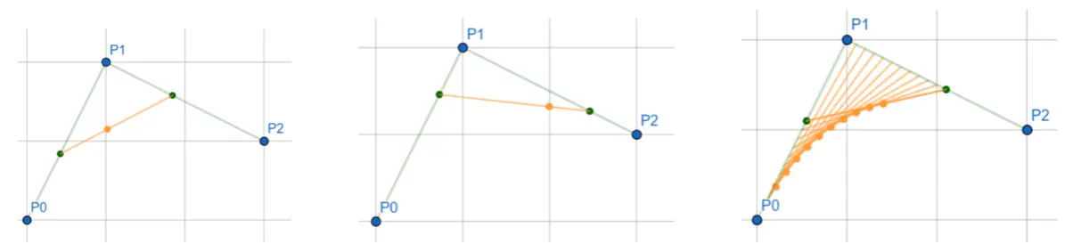
Releasing $t_{0}$ we have:

{\vec{B}}_{2, 0} (t) = (1 - t) (\begin{matrix} (1 - t) (- 1) \\ (1 - t) (2) + t (4) \end{matrix}) + t (\begin{matrix} t (5) \\ (1 - t) (4) + t (- 2) \end{matrix})

General Form:
Linear Bèzier curves:

{\vec{B}}_{1, i} (t) = (1 - t) \vec{P_{i}} + (t) \vec{P_{i + 1}}, i = 0, 1, \dots, n - 1.

These are ${\vec{P}}_{i} \to {\vec{P}}_{i + 1}$

Higher order curves:

{\vec{B}}_{j, i} (t) = (1 - t) \cdot {\vec{B}}_{j - 1, i} (t) + (t) \cdot {\vec{B}}_{j - 1, i + 1} (t), j = 2, 3, \dots, n; i = 0, 1, \dots, n - j .

These are the the at most $j^{t h}$ degree curve connecting ${\vec{P}}_{i} \to {\vec{P}}_{i + j}$ , via the control points ${\vec{P}}_{i + 1}, \dots {\vec{P}}_{i + j - 1}$ .

We will get:

B_{n, 0} (t) = \sum_{i = 0}^{n} (\binom{n}{i}) t^{i} (1 - t)^{n - 1} {\vec{P}}_{i}

(\binom{n}{i}) = \frac{n!}{i! (n - i)!}

Example:
The (at most) cubic Bézier curve with control points

{\vec{P}}_{0}, {\vec{P}}_{1}, {\vec{P}}_{2}, {\vec{P}}_{3}

is computed as follows:

First-order interpolation:

{\vec{B}}_{1, 0} (t) = (1 - t) {\vec{P}}_{0} + t {\vec{P}}_{1}

{\vec{B}}_{1, 1} (t) = (1 - t) {\vec{P}}_{1} + t {\vec{P}}_{2}

{\vec{B}}_{1, 2} (t) = (1 - t) {\vec{P}}_{2} + t {\vec{P}}_{3}

Second-order interpolation:

{\vec{B}}_{2, 0} (t) = (1 - t) {\vec{B}}_{1, 0} (t) + t {\vec{B}}_{1, 1} (t)

= (1 - t) [(1 - t) {\vec{P}}_{0} + t {\vec{P}}_{1}] + t [(1 - t) {\vec{P}}_{1} + t {\vec{P}}_{2}]

= (1 - t)^{2} {\vec{P}}_{0} + 2 t (1 - t) {\vec{P}}_{1} + t^{2} {\vec{P}}_{2}

{\vec{B}}_{2, 1} (t) = (1 - t) {\vec{B}}_{1, 1} (t) + t {\vec{B}}_{1, 2} (t)

= (1 - t) [(1 - t) {\vec{P}}_{1} + t {\vec{P}}_{2}] + t [(1 - t) {\vec{P}}_{2} + t {\vec{P}}_{3}]

= (1 - t)^{2} {\vec{P}}_{1} + 2 t (1 - t) {\vec{P}}_{2} + t^{2} {\vec{P}}_{3}

Third-order (cubic) interpolation:

{\vec{B}}_{3, 0} (t) = (1 - t) {\vec{B}}_{2, 0} (t) + t {\vec{B}}_{2, 1} (t)

= (1 - t) [(1 - t)^{2} {\vec{P}}_{0} + 2 t (1 - t) {\vec{P}}_{1} + t^{2} {\vec{P}}_{2}]

+ t [(1 - t)^{2} {\vec{P}}_{1} + 2 t (1 - t) {\vec{P}}_{2} + t^{2} {\vec{P}}_{3}]

= (1 - t)^{3} {\vec{P}}_{0} + 3 t (1 - t)^{2} {\vec{P}}_{1} + 3 t^{2} (1 - t) {\vec{P}}_{2} + t^{3} {\vec{P}}_{3}

Derivatives:

\frac{d}{d t} {\vec{B}}_{3, 0} (t) = - 3 (1 - t)^{2} {\vec{P}}_{0} + 3 [(1 - t)^{2} - 2 t (1 - t)] {\vec{P}}_{1} + 3 [2 t (1 - t) - t^{2}] {\vec{P}}_{2} + 3 t^{2} {\vec{P}}_{3}

Evaluating at ( t=0 ) and ( t=1 ):

\frac{d}{d t} {\vec{B}}_{3, 0} (t) |_{t = 0} = - 3 {\vec{P}}_{0} + 3 {\vec{P}}_{1} = 3 ({\vec{P}}_{1} - {\vec{P}}_{0})

\frac{d}{d t} {\vec{B}}_{3, 0} (t) |_{t = 1} = - 3 {\vec{P}}_{2} + 3 {\vec{P}}_{3} = 3 ({\vec{P}}_{3} - {\vec{P}}_{2})

These derivatives indicate that at $t = 0$ , the derivative of ${\vec{B}}_{3, 0}$ is in the direction of the segment from ${\vec{P}}_{0}$ to ${\vec{P}}_{1}$ , and at $t = 1$ , it is in the direction of the segment from ${\vec{P}}_{2}$ to ${\vec{P}}_{3}$ . The magnitude of these derivatives is exactly three times the magnitudes of the corresponding line segments.

Hermite Polynomial

General Osculating Polynomials

2. Given Data

3. Step-by-Step Computation

First Column: Function Values

First Divided Differences fi,1

Second Divided Differences fi,2

Third Divided Differences fi,3

Fourth Divided Differences fi,4

4. Key Observations

Bèzier Curves

Bezier Curve from P→0→P→n

First-order interpolation:

Second-order interpolation:

Third-order (cubic) interpolation:

Derivatives:

First Divided Differences $f_{i, 1}$

Second Divided Differences $f_{i, 2}$

Third Divided Differences $f_{i, 3}$

Fourth Divided Differences $f_{i, 4}$

Bezier Curve from ${\vec{P}}_{0} \to {\vec{P}}_{n}$